Google originally developed WebP as a lossy image format to supersede JPEG, one that was able to produce files smaller than a comparable-quality image file encoded as JPEG. Later updates to the format introduced the option of lossless compression, PNG-like alpha channel transparency, and GIF-like animation—all of which can be used alongside JPEG-style lossy compression. WebP is an unbelievably versatile format.
WebP's lossy compression algorithm is based on a method that the VP8 video codec uses to compress keyframes in videos. At a high level, it's similar to JPEG encoding: WebP operates in terms of "blocks" rather than individual pixels, and has a similar division between luminance and chrominance. WebP's luma blocks are 16x16, while chroma blocks are 8x8, and those "macroblocks" are further subdivided into 4x4 sub-blocks.
Where WebP differs radically from JPEG are in two features: "block prediction" and "adaptive block quantization."
Block Prediction
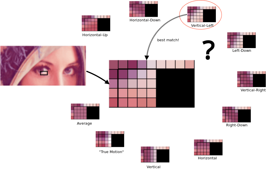
Block prediction is the process through which the contents of each chrominance and luminance block are predicted based on the values of their surrounding blocks—specifically the blocks above and to the left of the current block. As you might imagine, the algorithms that do this work are fairly complex, but to put it in plain language: "if there's blue above the current block, and blue to the left of the current block, assume this block is blue."
In truth, both PNG and JPEG also do this sort of prediction to some degree. WebP, however, is unique in that it samples the surrounding blocks' data and then attempts to populate the current block by way of several different "prediction modes", effectively trying to "draw" the missing part of the image. The results provided by each prediction mode are then compared to the real image data, and the closest predictive match is selected.

Even the closest predictive match isn't going to be completely right, of course, so the differences between the predicted and actual values of that block are encoded in the file. When decoding the image, the rendering engine uses the same data to apply the same predictive logic, leading to the same predicted values for each block. The difference between the prediction and the expected image that was encoded in the file is then applied over the predictions—similar to how a Git commit represents a differential patch that gets applied over the local file, rather than a brand new copy of the file.
To illustrate: rather than dig into the complex math involved in the true predictive algorithm, we'll invent a WebP-like encoding with a single prediction mode, and use it to efficiently relay a grid of numbers the way we did with the legacy formats. Our algorithm has a single prediction mode, which we'll call "prediction mode one:" the value of each block is the sum of the values of the blocks above it and to the left of it, starting with 1.
Now, say we're starting with the following real image data:
111151111
122456389
Using our predictive model to determine the contents of a 2x9 grid, we would get the following result:
111111111
123456789
Our data is a good fit for the predictive algorithm we've invented—the predicted data is a close match to our real data. Not a perfect fit, of course—the actual data has several blocks that are different from the predicted data. So, the encoding we send includes not just the prediction method to use, but a diff of any blocks that should differ from their predicted values:
_ _ _ _ +4 _ _ _ _
_ _ -1 _ _ _ -4 _ _
Put in the same kind of plain language as some of the legacy format encodings we've discussed:
2x9 grid using prediction mode one. +4 to 1x5, -1 to 2x3, -4 to 2x7.
The end result is an unbelievably efficient encoded file.
Adaptive block quantization
JPEG compression is a blanket operation, applying the same level of quantization to every block in the image. In an image with a uniform composition, that certainly makes sense—but real-world photographs aren't any more uniform than the world around us. In practice, this means that our JPEG compression settings are determined not by the high frequency details—where JPEG compression excels—but by the parts of our image where compression artifacts are most likely to appear.

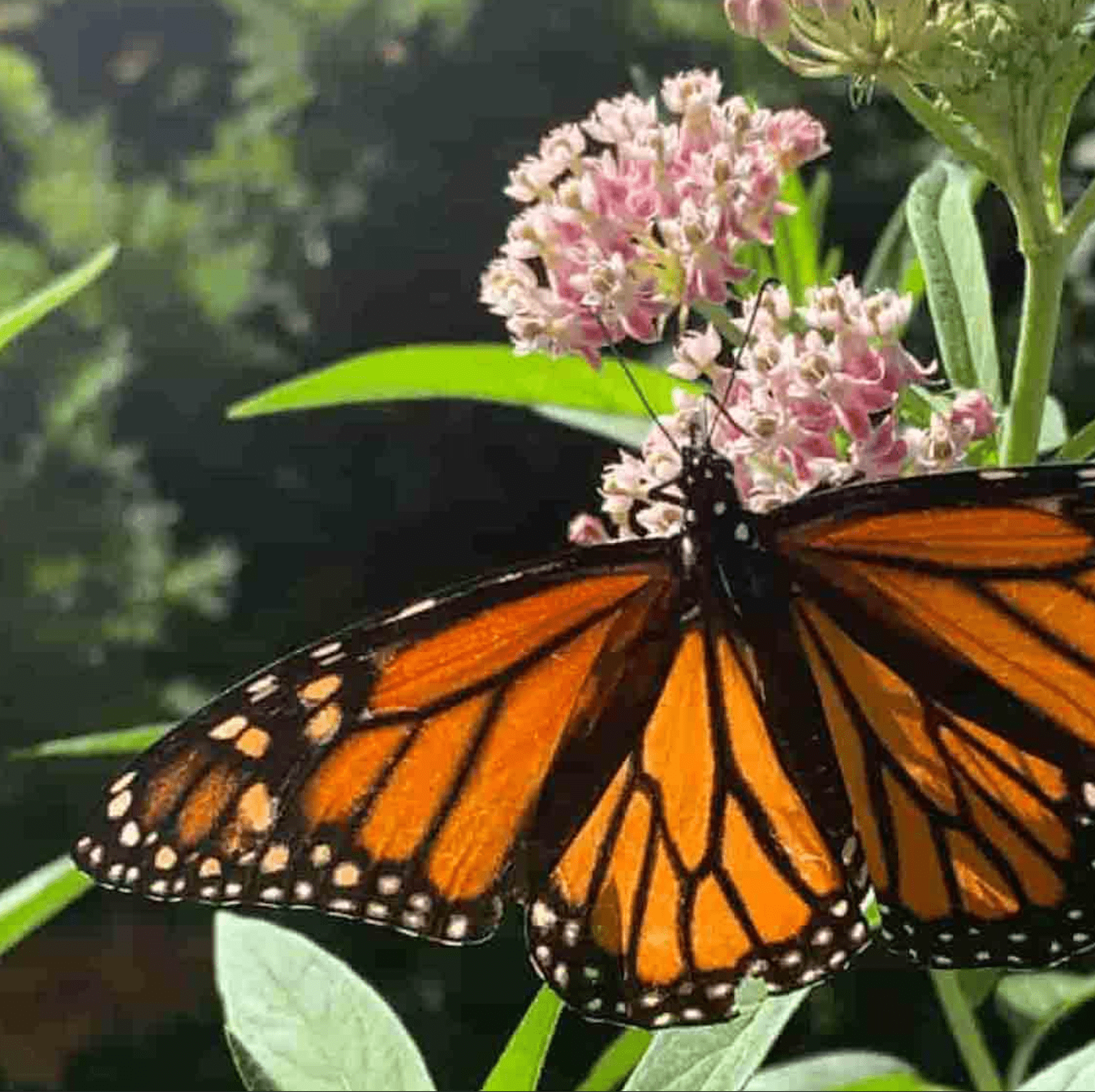
As you can see in this exaggerated example, the wings of the monarch in the foreground look relatively sharp—a little grainy when compared with the high-resolution original, but certainly not noticeable without the original to compare with it. Likewise, the detailed inflorescence of the milkweed, and the leaves in the foreground—you and I may see traces of compression artifacts with our trained eyes, but even with the compression dialed up well beyond reasonable levels things in the foreground still look passably crisp. The low-frequency information at the top left of the picture—the blurry green backdrop of leaves—looks terrible. Even an untrained viewer would immediately notice the quality issue—the subtle gradients in the background are rounded down to jagged, solid-color blocks.
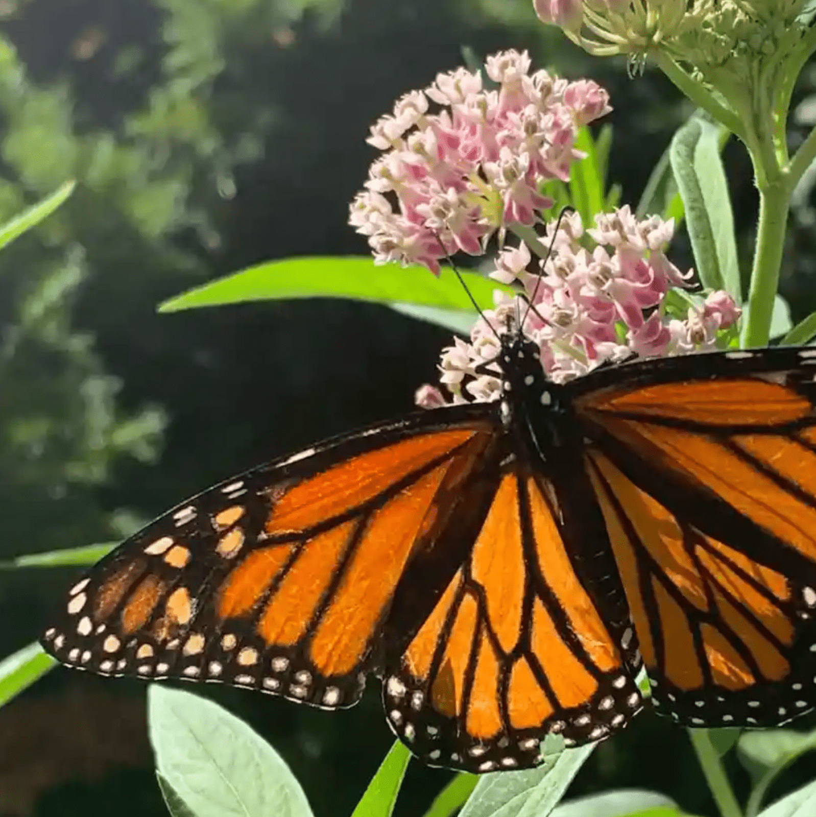
In order to avoid this, WebP takes an adaptive approach to quantization: an image is broken into up to four visually similar segments, and compression parameters for those segments are tuned independently. Using the same outsized compression with WebP:

The size of both these image files is about the same. The quality is about the same when we look at the monarch's wings—you can spot a few tiny differences in the end result if you look very, very closely, but no real difference in overall quality. In the WebP, the flowers of the milkweed are just a little sharper—again, likely not enough to be noticeable unless you're comparing the two side-by-side and really looking for differences in quality, the way we are. The background is a different story altogether: it has barely a trace of JPEG's glaringly obvious artifacts. WebP gives us the same file size, but a much higher quality image—give or take a few tiny details that our psychovisual systems wouldn't be able to detect if we weren't comparing the two so closely.
Using WebP
The internals of WebP might be considerably more complex than JPEG encoding, but just as simple for the purpose of our daily work: all the complexity of WebP's encoding is standardized around a single "quality" value—expressed from 0–100, just like JPEG. And once again, that's not to say that you're limited to a single overarching "quality" setting. You can—and should—tinker with all the fine details of WebP encoding, if only to gain a better understanding of how these normally-invisible settings can impact file size and quality.
Google offers a cwebp command line encoder that allows you to convert or compress individual files or entire directories of images:
$ cwebp -q 80 butterfly.jpg -o butterfly.webp

Saving file 'butterfly.webp'
File:   butterfly.jpg
Dimension: 1676 x 1418
Output: 208418 bytes Y-U-V-All-PSNR 41.00 43.99 44.95   41.87 dB
        (0.70 bpp)
block count:    intra4:     7644  (81.80%)
               Intra16:     1701  (18.20%)
               Skipped:       63  (0.67%)
bytes used:  header:            249  (0.1%)
              mode-partition:  36885  (17.7%)
Residuals bytes  |segment 1|segment 2|segment 3|segment 4|  total
macroblocks:     |       8%|      22%|      26%|      44%|   9345
quantizer:       |      27 |      25 |      21 |      13 |
filter level:    |       8 |       6 |      19 |      16 |
And if you're not inclined toward the command line, Squoosh will serve us just as well for encoding WebP. It gives us the option of side-by-side comparisons between different encodings, settings, quality levels, and differences in file size from JPEG encoding.
